Quickstart

Note

You can download this quickstart script here.

This tutorial shows how to calculate light rays between curves calculated from scratch, meaning neither curve data nor configuration files need to be defined prior to starting the tutorial. If the user already created curves saved as h5 files, please refer to the tutorial on how to import existing curve data.

The premise of the emitter-observer problem is having one curve defining the emitter and one curve defining the observer. At first, supply corresponding initial conditions and the spacetime metric in which curves should be calculated; refer to the source code for the dictionary of implemeted spacetime metrics.

Initial conditions and the spacetime metric are supplied as a dictionary of the following form:

config = {
    'Curve_1': {
        'proper_times': {'time_initial': 0, 'time_final': 7000.0},
        'initial_event': {
            'x0': 0,
            'radius': 6971000.0,
            'theta': 1.5707963267948966,
            'phi': 0
        },
        'initial_velocity': {
            'velocity_radial': 0,
            'velocity_polar': 0,
            'velocity_azimuthal': 0.00110815,
        },
    },
    'Curve_2': {
        'proper_times': {'time_initial': 0, 'time_final': 7000.0},
        'initial_event': {
            'x0': 0,
            'radius': 7071000.0,
            'theta': 1.5707963267948966,
            'phi': 0
        },
        'initial_velocity': {
            'velocity_radial': 0,
            'velocity_polar': 0,
            'velocity_azimuthal': 0.00110815,
        }
    },
    'Metric': {
        'name': 'Schwarzschild',
        'params': {'multipole_moments': [398600441500000.0]},
    },
}

Each curve i with index i going over 1 and 2 has three keys:

• proper_times defining the initial and final proper time value of the curve,

• initial_event defining the four-coordinates of the curve’s initial event,

• initial_velocity defining the curve’s spatial (three)-velocity at the initial event.

The spacetime metric is supplied via

• name defining the line element,

• multipole_moments defining the gravitating object’s parameters.

The initial_conditions_calc function calculates the four-velocities at the initial events from the given config dictionary and returns the events with their corresponding four-velocity:

from greopy.initial_conditions import initial_conditions_calc

event_1, velocity_1, event_2, velocity_2 = initial_conditions_calc(
        config,
)

Each event with their initial four-velocity forms an initial value problem that is solved with the geodesic_calc function; the returned curves are the emitter and receiver that will be exchanging light signals:

from greopy.orbit_calc import geodesic_calc

emission_curve_data, receiver_curve_data = geodesic_calc(
config,
(event_1, velocity_1, event_2, velocity_2),
)

The variables *_curve_data each contain a pandas DataFrame where every row holds the event and respective four-velocity of each curve step. Since geodesic_calc’s default argument step_numbers was left blank, it defaults to 600 steps along both curves.

If emission_curve_data would be used unaltered, the following code would calculate 600 light rays, one for each curve step. For this simple example, only a couple of light signals should be exchanged. Therefore reduce the number of rows in the DataFrame to reduce number of light rays to be calculated:

emission_curve_reduced = emission_curve_data[0:600:150]

This results in four events numbered 0, 150, 300, 450; a light ray to be calculated at each one.

The light signals can now be calculated via the eop_solver function, given the config and the two previously calculated curves:

from greopy.emitter_observer_problem import eop_solver

light_rays = eop_solver(
        config,
        emission_curve_reduced,
        receiver_curve_data,
        hypersurface_approximation=True,
        euclidean_approximation=True,
)

This function calculates a light ray for each emission event that intersects the receiver curve at some reception event and saves the light curve in a pandas DataFrame. It has some parameters concerning computational efficiency that can be adapted for different satellite scenarios, in this case:

• hypersurface_approximation enables an initial guess for the correct celestial angles by approximating them with a geodesic in the x0=const. hypersurface,

• euclidean_approximation enables calculating the distance between two events with the euclidean definition instead of the general-relativistic definition [1].

Note

The multiprocessing flag enables multiprocessing, i.e. light rays at multiple events can be calculated simultaneously depending on the number of CPU cores available. This can greatly reduce computation time.

However the default start method for multiprocessing is different on different operating systems. When enabling multiprocessing on Windows or macOS, please add the following line of code to the beginning of your (quickstart) script to change the default method from ‘spawn’ to ‘fork’:

import multiprocessing
multiprocessing.set_start_method('fork')

Since Linux uses the ‘fork’ method by default, these lines can be omitted.

For more information on all the function parameters, refer to the documentation

The resulting light_rays lists all indexed DataFrames.

Optionally, the results (emitter-, receiver- and light curves) can be visualised via the eop_plot function. In this case, displaying the resulting plot without saving it requires a Matplotlib backend. One example could be using the QtAgg interactive backend, which requires PyQt that can be installed via pip.

The result may look like this:

import matplotlib.pyplot as plt
from greopy.emitter_observer_solution_plot import eop_plot

eop_plot(emission_curve_data, receiver_curve_data, light_rays)
plt.show()

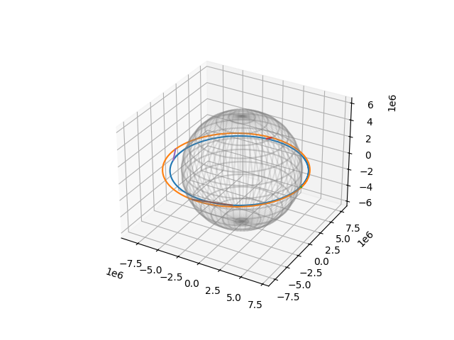
Emission curve (blue) emits light signals that intersect receiver curve (orange).

[1]

Note that the final distance calculation (as a check) with the result light ray will always be done with the general-relativistic definition of distance.