Quickstart

This tutorial shows how to calculate light rays between curves calculated from scratch, meaning neither curve data nor configuration files need to be defined prior to starting the tutorial.

import numpy as np
import matplotlib.pyplot as plt
from greopy.initial_conditions import initial_conditions_calc
from greopy.orbit_calc import geodesic_calc
from greopy.emitter_observer_problem import eop_solver
from greopy.emitter_observer_solution_plot import eop_plot

Initial conditions and the spacetime metric are supplied as a dictionary of the following form:

config = {
    'Curve_1': {
        'proper_times': {'time_initial': 0, 'time_final': 7000.0},
        'initial_event': {
            'x0': 0,
            'radius': 6971000.0,
            'theta': np.pi / 2,
            'phi': 0
        },
        'initial_velocity': {
            'velocity_radial': 0,
            'velocity_polar': 0,
            'velocity_azimuthal': 0.00110815,
        },
    },
    'Curve_2': {
        'proper_times': {'time_initial': 0, 'time_final': 7000.0},
        'initial_event': {
            'x0': 0,
            'radius': 7071000.0,
            'theta': np.pi / 2,
            'phi': 0
        },
        'initial_velocity': {
            'velocity_radial': 0,
            'velocity_polar': 0,
            'velocity_azimuthal': 0.00110815,
        }
    },
    'Metric': {
        'name': 'Schwarzschild',
        'params': {'multipole_moments': [398600441500000.0]},
    },
}

The initial_conditions_calc function is used to calculate the four-velocities at the initial events from the given config dictionary and returns the events with their corresponding four-velocity:

event_1, velocity_1, event_2, velocity_2 = initial_conditions_calc(config)

Each event with their initial four-velocity forms an initial value problem that is solved with the geodesic_calc function; the returned curves are the emitter and receiver that will be exchanging light signals:

emission_curve_data, receiver_curve_data = geodesic_calc(
    config,
    (event_1, velocity_1, event_2, velocity_2),
)

Reduce the number of rows in the DataFrame to reduce number of light rays to be calculated:

emission_curve_reduced = emission_curve_data[0:600:150]

The light signals can now be calculated via the eop_solver function, given the config and the two previously calculated curves:

light_rays = eop_solver(config,
                        emission_curve_reduced,
                        receiver_curve_data,
                        hypersurface_approximation=True,
                        euclidean_approximation=True)

The seed for this computation is 44351

Optionally, the results can be visualised via the eop_plot function:

eop_plot(emission_curve_data, receiver_curve_data, light_rays)

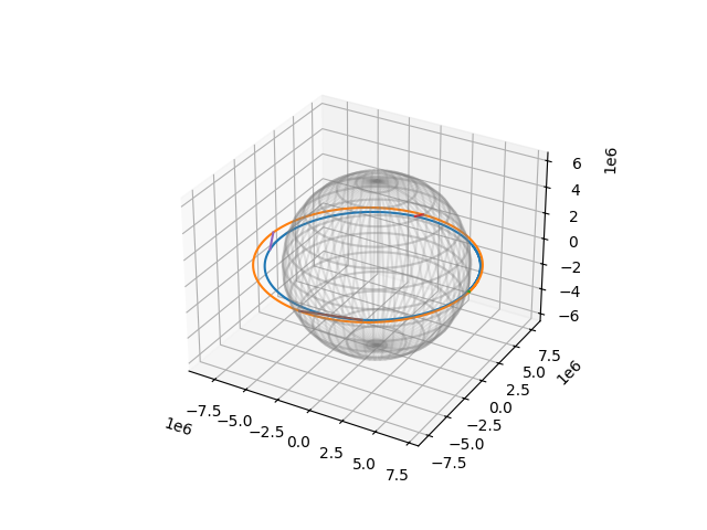
This plots the emission, receiver and light ray curves. From here, the plot can either be shown or saved via the corresponding matplotlib functions. For this example, the result will just be shown without saving it, which requires a Matplotlib backend, see https://matplotlib.org/stable/users/explain/figure/backends.html for more information:

plt.show()